Streaming data to disk
The example IOCs in quadEM load the file ADCore/iocBoot/commonPlugins.cmd. This provides all the standard file plugins, including HDF5, netCDF, and TIFF. These can be used to stream the quadEM data to disk, with no limit on the duration except for disk file size.
As explained in the Plugins section, the NDArray callbacks to plugins occur each time NumAverage_RBV samples have been received from the device. Callbacks on address 11 contain all the data items, and the NDArray dimensions are [11, NumAverage_RBV] for each NDArray callback.
This is the medm screen for the HDF5 plugin used with the TetrAMM. The TetrAMM is configured with ValuesPerRead=5, so it is sending data at 20 kHz. AveragingTime is set to 0.1 seconds, so NumAverage_RBV is 2000.
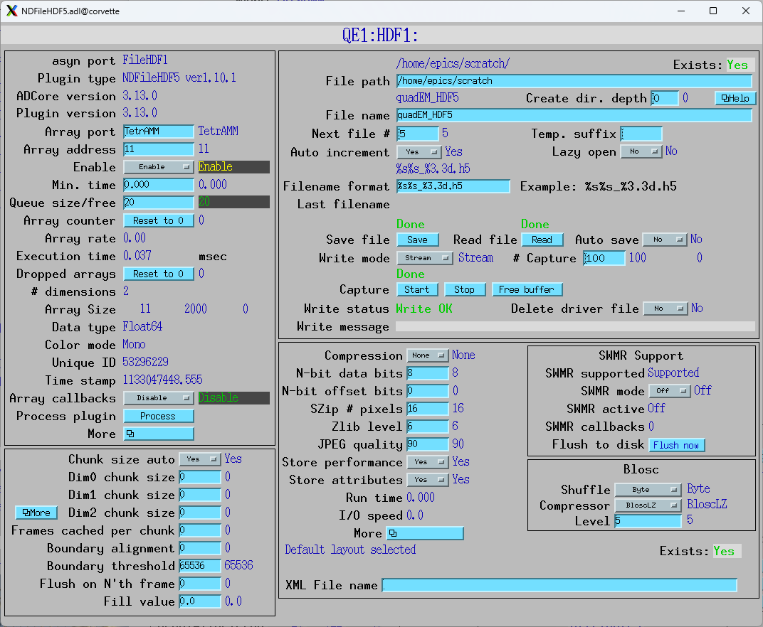
The Array address in the plugin is set to 11, so it is receiving all 11 data items. FileWriteMode is set to Stream, so it will stream the NDArrays to the HDF5 file as they arrive. NumCapture is set to 200, so it will collect 200 arrays, each with 0.1 second of data giving a total of 20 seconds saved to disk. Pressing the Start button starts the streaming.
The resulting file, quadEM_HDF5_001.h5, is 34 MB.
This is the result of the Linux h5dump –contents on that file
(base) [epics@corvette scratch]$ h5dump --contents quadEM_HDF5_001.h5
HDF5 "quadEM_HDF5_001.h5" {
FILE_CONTENTS {
 group      /
 group      /entry
 group      /entry/data
 dataset    /entry/data/data
 group      /entry/instrument
 group      /entry/instrument/NDAttributes
 dataset    /entry/instrument/NDAttributes/NDArrayEpicsTSSec
 dataset    /entry/instrument/NDAttributes/NDArrayEpicsTSnSec
 dataset    /entry/instrument/NDAttributes/NDArrayTimeStamp
 dataset    /entry/instrument/NDAttributes/NDArrayUniqueId
 group      /entry/instrument/detector
 group      /entry/instrument/detector/NDAttributes
 dataset    /entry/instrument/detector/data -> /entry/data/data
 group      /entry/instrument/performance
 dataset    /entry/instrument/performance/timestamp
 }
}
The streamed data is in dataset /entry/data/data. This is the output of h5dump –header, looking at just that dataset.
   DATASET "data" {
      DATATYPE  H5T_IEEE_F64LE
      DATASPACE  SIMPLE { ( 200, 2000, 11 ) / ( 200, 2000, 11 ) }
      ATTRIBUTE "NDArrayDimBinning" {
         DATATYPE  H5T_STD_I32LE
         DATASPACE  SIMPLE { ( 2 ) / ( 2 ) }
      }
      ATTRIBUTE "NDArrayDimOffset" {
         DATATYPE  H5T_STD_I32LE
         DATASPACE  SIMPLE { ( 2 ) / ( 2 ) }
      }
      ATTRIBUTE "NDArrayDimReverse" {
         DATATYPE  H5T_STD_I32LE
         DATASPACE  SIMPLE { ( 2 ) / ( 2 ) }
      }
      ATTRIBUTE "NDArrayNumDims" {
         DATATYPE  H5T_STD_I32LE
         DATASPACE  SCALAR
      }
      ATTRIBUTE "signal" {
         DATATYPE  H5T_STD_I32LE
         DATASPACE  SCALAR
      }
   }
}
It is IEEE 64-bit little-endian, with dimensions [200,2000,11]. In HDF5 convention the last array index is the fastest varying.
Saving all 11 data items is somewhat wastefull, since everything else can be calculated from just the 4 currents, which are the first 4 items in the arrays. We can save disk space by only saving the currents by using an ROI plugin between the quadEM driver and the HDF5 plugin.
This is the medm screen for an ROI plugin which gets its data on address 11 from the TetrAMM port. It is configured with a start of 0 and size of 4 on the first array dimension, and so will select only the 4 currents. The second dimension is set to auto size = Yes, so it will automatically select all elements in the second dimension, even if NumAverage_RBV changes.

The HDF5 plugin is changed to have its array port be ROI1, and the array address to be 0. Note that the NDArrays being received are now [4, 2000].
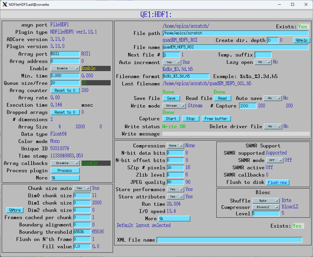
The filename is changed to quadEM_HDF5_ROI_001.h5. The resulting file size is 13 MB.
The following is an IDL program to process the data in quadEM_HDF5_001.h5. The program does the following:
Reads the dataset /entry/data/data into a variable called
data.Displays information about
data.Reformats
datafrom a 3-D array with dimensions [11, 2000, 200] to a 2-D array with dimensions [11, 400000].Extracts the SumAll data into a variable called
sum_all, which the 6’th column ofdata.Compute a
timearray variable which is the time of each sample. It is 400000 points with 50 microseconds per point.Plots the first 0.5 seconds (1000 points) of
sum_allvstime.Computes the absolute value of the FFT of the
sum_allvariable, which is the power spectrum.Sets the first element (0 frequency, i.e. DC offset) to 0.
Computes the frequency axis, which is 200000 points going from 0 to the Nyquist freqency of 10 kHz.
Plots the power spectrum vs frequency. Plots only the first 20000 points, which is 0 to 1 kHz, on a vertical log scale.
This is the IDL code:
; Program to read HDF5 file for streamed quadEM data, plot it
data = h5_getdata('J:\epics\scratch\quadEM_HDF5_001.h5', '/entry/data/data')
help, data
; Convert from a 3-D array [11, 2000, 200] to a 2-D array [11, 400000]
data = reform(data, 11, 400000)
; Extract the SumAll data
sum_all = data[6, *]
; Compute the time axis, 50 microseconds/sample
time = findgen(400000) * 50e-6
; Plot the first 0.5 second of data
p1 = plot(time[0:9999], sum_all[0:9999], xtitle='Time (s)', ytitle='Sum of all diodes (nA)', $
          title='Time Series', color='blue')
p1.save, 'IDL_HDF5_time_plot.png'
; Compute the FFT
f = fft(sum_all)
; Take the absolute value, first half of array
f_abs = (abs(f))[0:199999]
; Set the DC offset to 0
f_abs[0] = 0
; Compute the frequency axis. The sampling rate is 20 kHz so the Nyquist frequency is 10 kHz
freq = findgen(200000)/199999. * 10000.
; Plot the data out to 1 kHz
p2 = plot(freq[0:19999], f_abs[0:199999], xtitle='Frequency (Hz)', ytitle='SumAll Intensity', $
          title='Power Spectrum', color='red', /ylog, yrange=[.01,100])
p2.save, 'IDL_HDF5_frequency_plot.png'
end
This is the output when the program is compiled and run:
IDL> .compile -v 'C:\Scratch\plot_quadem.pro'
IDL> .go
DATA            DOUBLE    = Array[11, 2000, 200]
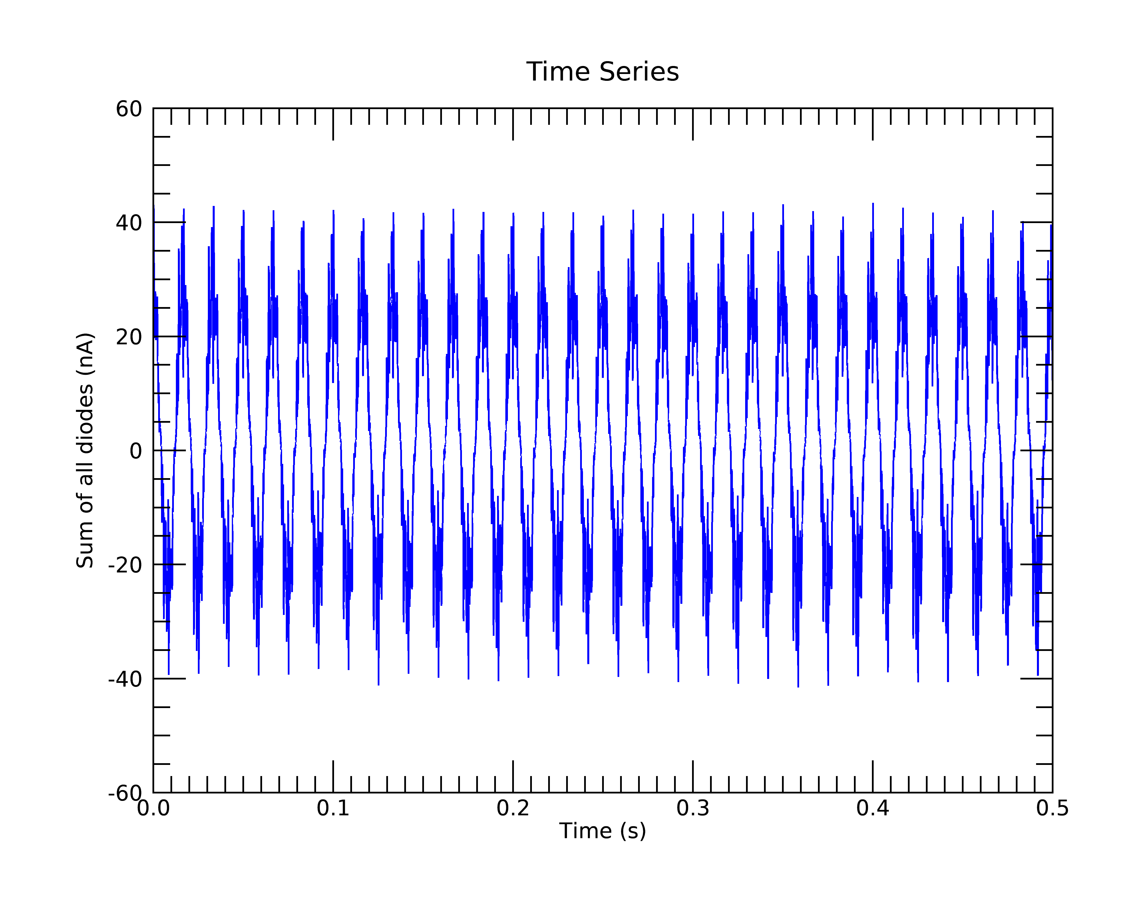
This is the time-series plot. The data are highly periodic because the photodiodes were illuminated by fluorescent lights.
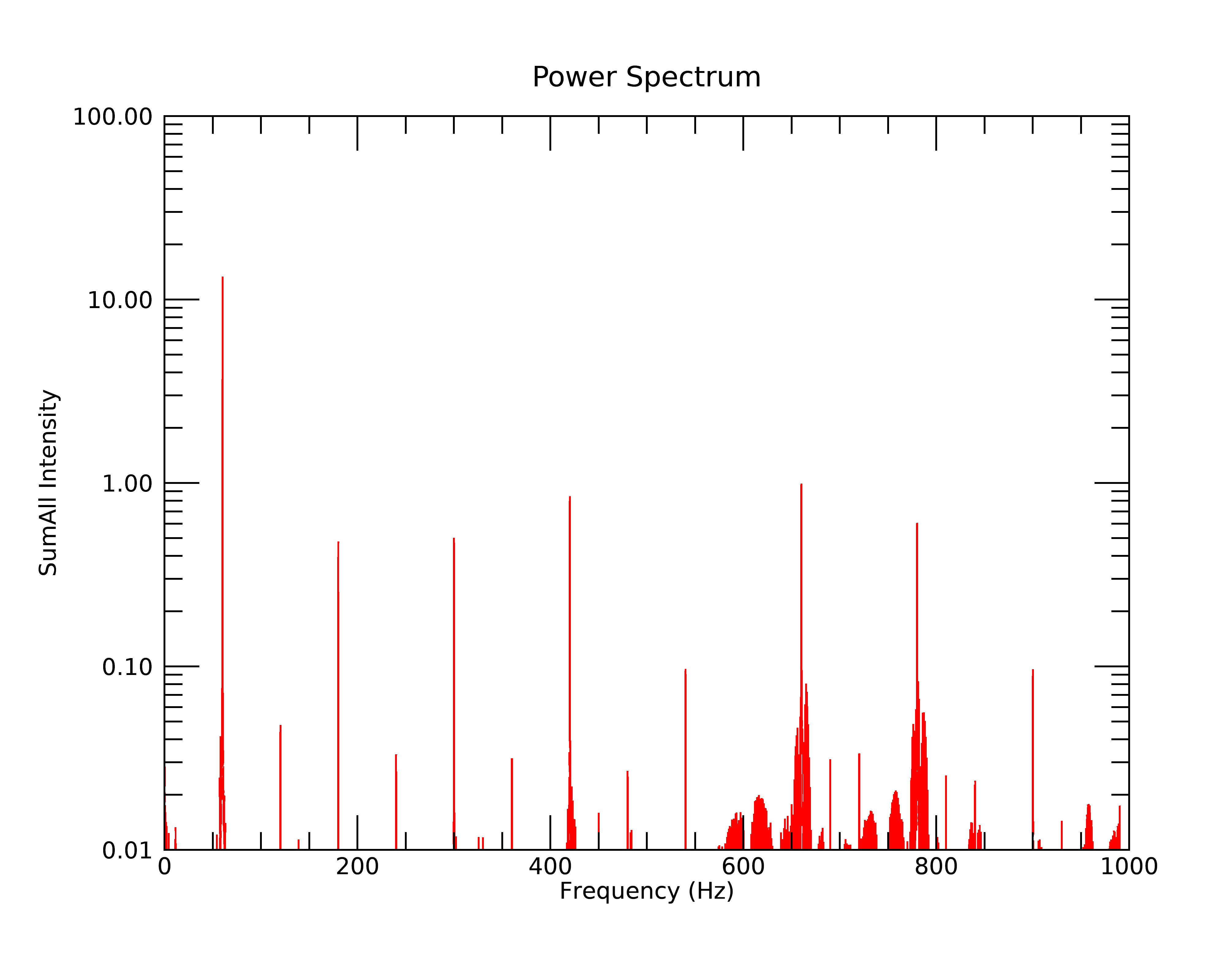
This is the frequency plot. The peaks are almost exclusively 60 Hz and its odd and even harmonics. The odd harmonics are ~10-100 times less than 60 Hz, and the even harmonics are ~100-1000 times less than 60 Hz.
Using Python, the data processing would be nearly identical, but with a few differences due to array and FFT conventions:
import numpy as np
import h5py

# Windows/MacOS: pip install wxmplot
# Linux: canda install -c conda-forge wxpython && pip install wxmplot
from wxmplot.interactive import plot

h5root = h5py.File('quadem_HDF5_001.h5')
data = h5root['/entry/data/data'][()]
ny, nx, nchans = data.shape  # = (200, 2000, 11)
npts = ny*nx
data.shape = (npts, 11)
sum_all = data[:, 6]

sample_time = 50e-6
time = np.arange(npts)*sample_time

# Plot the first 0.5 second of data
p1 = plot(time[:10000], sum_all[:10000],
          xlabel='Time (s)', ylabel='Sum of all diodes (nA)', title='Time Series')
p1.save_figure('Py_HDF5_time_plot.png')

# Compute the FFT: note that for numpy.fft, the normalization is set with
#  'norm', which can be one of 'backward', 'forward, or 'ortho'.
#  'backward' is the NumPy default, 'forward' matches the IDL default.
f = np.fft.fft(sum_all, norm='forward')
# or one of:
# f = np.fft.fft(sum_all) / npts
# f = np.fft.fft(sum_all, norm='ortho') / np.sqrt(npts)

# Take the absolute value, first half of array
nfft = npts//2
f_abs = abs(f)[:nfft]

# Set the DC offset to 0
f_abs[0] = 0

# Compute the frequency axis.
# Note: The sampling rate is 20 kHz so the Nyquist frequency is 10 kHz
freq = np.arange(nfft)/(nfft*2*sample_time)
# or
# freq = np.fft.fftfreq(npts, sample_time)

# Plot the power spectrum out to 1 kHz
p2 = plot(freq[:20000], f_abs[:20000], ymin=0.01, ymax=100, ylog_scale=True,
          xlabel='Frequency (Hz)', ylabel=r'SumAll Intensity', color='red',
          title='Power Spectrum',  win=2)

p2.save_figure('Py_HDF5_frequency_plot.png')
This will make a time-series plot of:

and a frequency plot of:
